Core Concepts
Broad technical terms
| Object | Description |
| argset | A named list containing a set of arguments. |
| analysis |
These are the fundamental units that are scheduled in
|
| plan |
This is the overarching “scheduler”:
|
Different types of plans
| Plan Type | Description |
| Single-function plan | Same action function applied multiple times with different argsets applied to the same datasets. |
| Multi-function plan | Different action functions applied to the same datasets. |
Plan Examples
| Plan Type | Example |
| Single-function plan | Multiple strata (e.g. locations, age groups) that you need to apply the same function to to (e.g. outbreak detection, trend detection, graphing). |
| Single-function plan | Multiple variables (e.g. multiple outcomes, multiple exposures) that you need to apply the same statistical methods to (e.g. regression models, correlation plots). |
| Multi-function plan | Creating the output for a report (e.g. multiple different tables and graphs). |
Single-function plan
Use this approach in one of these two cases:
- You have multiple strata (e.g. locations, age groups) that you need to apply the same statistical methods to.
- You have multiple variables (e.g. multiple exposures, multiple outcomes) that you want to apply the same statistical methods to.
When you apply the same function multiple times, add the argsets first. Then apply the analysis function, just before you run the analyses.
Multiple strata
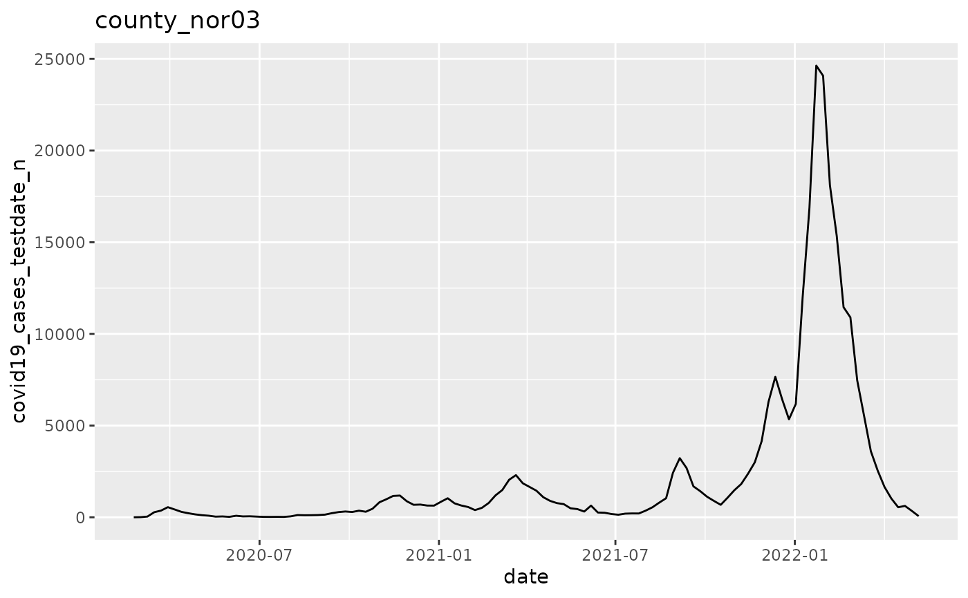
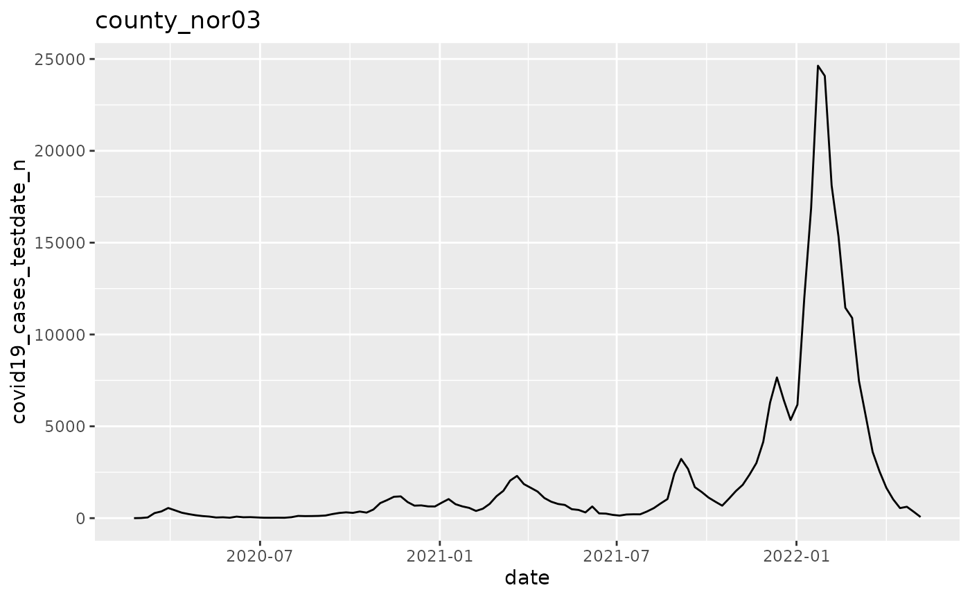
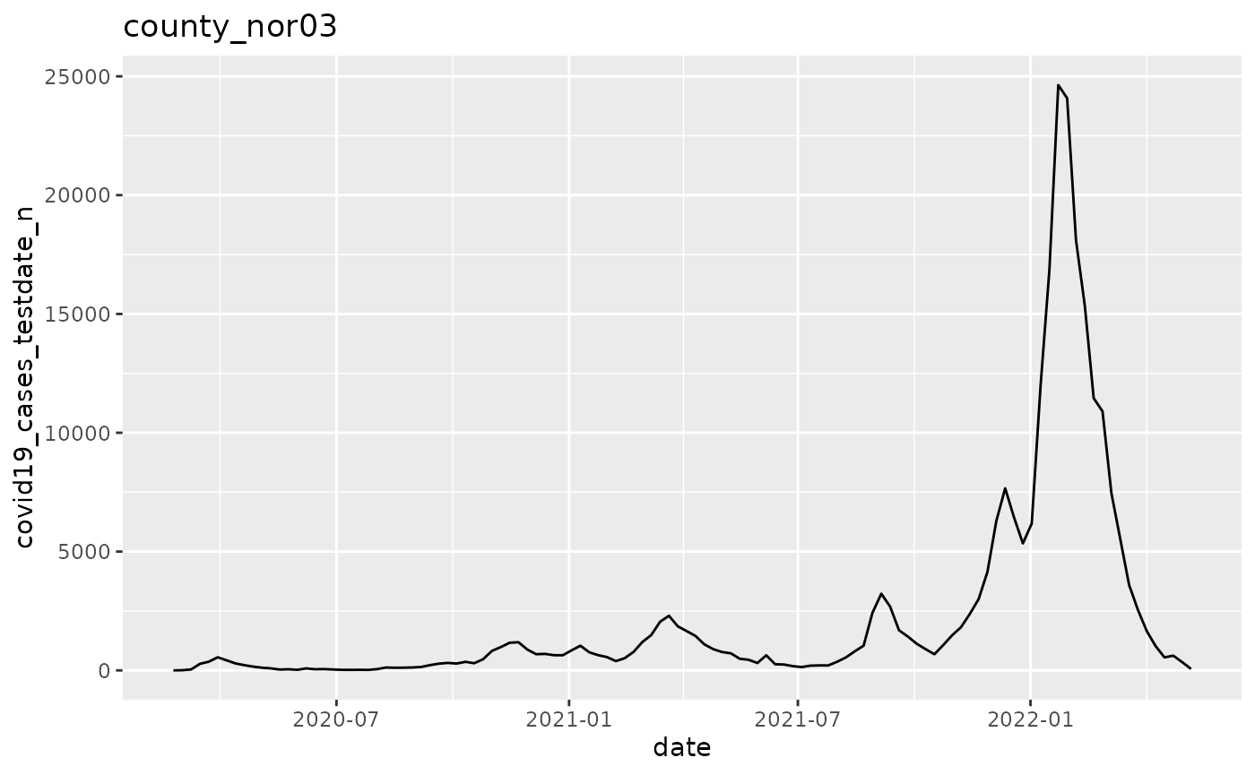
This example loops through multiple geographical locations. It applies a graphing function to the data from each of those locations.
##
## Attaching package: 'data.table'
## The following object is masked from 'package:base':
##
## %notin%
# We begin by defining a new plan
p <- plnr::Plan$new()
# Data function
data_fn <- function(){
return(plnr::nor_covid19_cases_by_time_location)
}
# We add sources of data
# We can add data directly
p$add_data(
name = "covid19_cases",
fn_name = "data_fn"
)
p$get_data()## $covid19_cases
## granularity_time granularity_geo country_iso3 location_code border
## <char> <char> <char> <char> <int>
## 1: day county nor county_nor03 2020
## 2: day county nor county_nor03 2020
## 3: day county nor county_nor03 2020
## 4: day county nor county_nor03 2020
## 5: day county nor county_nor03 2020
## ---
## 11024: isoweek nation nor nation_nor 2020
## 11025: isoweek nation nor nation_nor 2020
## 11026: isoweek nation nor nation_nor 2020
## 11027: isoweek nation nor nation_nor 2020
## 11028: isoweek nation nor nation_nor 2020
## age sex isoyear isoweek isoyearweek season seasonweek calyear
## <char> <char> <int> <int> <char> <char> <num> <int>
## 1: total total 2020 8 2020-08 2019/2020 31 2020
## 2: total total 2020 8 2020-08 2019/2020 31 2020
## 3: total total 2020 8 2020-08 2019/2020 31 2020
## 4: total total 2020 9 2020-09 2019/2020 32 2020
## 5: total total 2020 9 2020-09 2019/2020 32 2020
## ---
## 11024: total total 2022 14 2022-14 2021/2022 37 NA
## 11025: total total 2022 15 2022-15 2021/2022 38 NA
## 11026: total total 2022 16 2022-16 2021/2022 39 NA
## 11027: total total 2022 17 2022-17 2021/2022 40 NA
## 11028: total total 2022 18 2022-18 2021/2022 41 NA
## calmonth calyearmonth date covid19_cases_testdate_n
## <int> <char> <Date> <int>
## 1: 2 2020-M02 2020-02-21 0
## 2: 2 2020-M02 2020-02-22 0
## 3: 2 2020-M02 2020-02-23 0
## 4: 2 2020-M02 2020-02-24 0
## 5: 2 2020-M02 2020-02-25 0
## ---
## 11024: NA <NA> 2022-04-10 6888
## 11025: NA <NA> 2022-04-17 3635
## 11026: NA <NA> 2022-04-24 3764
## 11027: NA <NA> 2022-05-01 2243
## 11028: NA <NA> 2022-05-08 502
## covid19_cases_testdate_pr100000
## <num>
## 1: 0.000000
## 2: 0.000000
## 3: 0.000000
## 4: 0.000000
## 5: 0.000000
## ---
## 11024: 126.961423
## 11025: 67.001274
## 11026: 69.379036
## 11027: 41.343564
## 11028: 9.252996
##
## $hash
## $hash$current
## [1] "cbb5d442160f26df4c2d9a4fec794fd7"
##
## $hash$current_elements
## $hash$current_elements$covid19_cases
## [1] "7f1b0a581386e75e907bffd94938a3a7"
## [1] "county_nor03" "county_nor11" "county_nor15" "county_nor18" "county_nor30"
## [6] "county_nor34" "county_nor38" "county_nor42" "county_nor46" "county_nor50"
## [11] "county_nor54" "nation_nor"
p$add_argset_from_list(
plnr::expand_list(
location_code = location_codes,
granularity_time = "isoweek"
)
)
# Examine the argsets that are available
p$get_argsets_as_dt()## name_analysis index_analysis location_code
## <char> <int> <list>
## 1: 1a83f564-1eb1-4be8-b5b5-81ab1c8e836f 1 county_nor03
## 2: 6d3fb97d-350d-4567-b359-d92586d321f2 2 county_nor11
## 3: 06934ce6-0ded-4b69-bc98-a9925555cf04 3 county_nor15
## 4: 9e76beb7-9f95-4c6d-8b46-d5063886def2 4 county_nor18
## 5: 49fbbc71-0a9f-4616-90fb-f0600cd0de32 5 county_nor30
## 6: 599ecf4a-9d1f-482f-90df-61dfa64d19a0 6 county_nor34
## 7: c506c7fc-414d-4d3c-8e64-2f204267cfc3 7 county_nor38
## 8: 9b36932c-4c3d-4dea-96c7-29d78bda117d 8 county_nor42
## 9: e0e520d2-347b-46de-b642-f32d41c8b3ad 9 county_nor46
## 10: ff684952-4ba5-411a-9ccb-1f74332d9e1e 10 county_nor50
## 11: 8bb8be9e-1a06-4557-af1e-ce09744400bd 11 county_nor54
## 12: 377ce844-e72d-443c-b4b5-60ef8fa06e7f 12 nation_nor
## granularity_time
## <list>
## 1: isoweek
## 2: isoweek
## 3: isoweek
## 4: isoweek
## 5: isoweek
## 6: isoweek
## 7: isoweek
## 8: isoweek
## 9: isoweek
## 10: isoweek
## 11: isoweek
## 12: isoweek
# We can then add a simple analysis that returns a figure:
# To do this, we first need to create an action function
# (takes two arguments -- data and argset)
action_fn <- function(data, argset){
if(plnr::is_run_directly()){
data <- p$get_data()
argset <- p$get_argset(1)
}
pd <- data$covid19_cases[
location_code == argset$location_code &
granularity_time == argset$granularity_time
]
q <- ggplot(pd, aes(x=date, y=covid19_cases_testdate_n))
q <- q + geom_line()
q <- q + labs(title = argset$location_code)
q
}
p$apply_action_fn_to_all_argsets(fn_name = "action_fn")
p$run_one(1)
q <- p$run_all()
q[[1]]
q[[2]]
Multiple variables
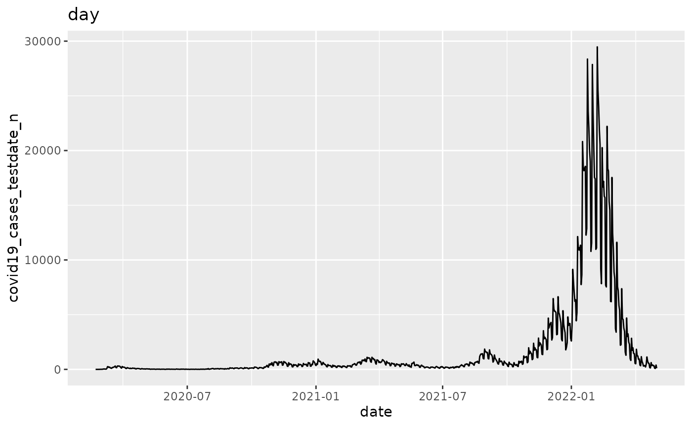
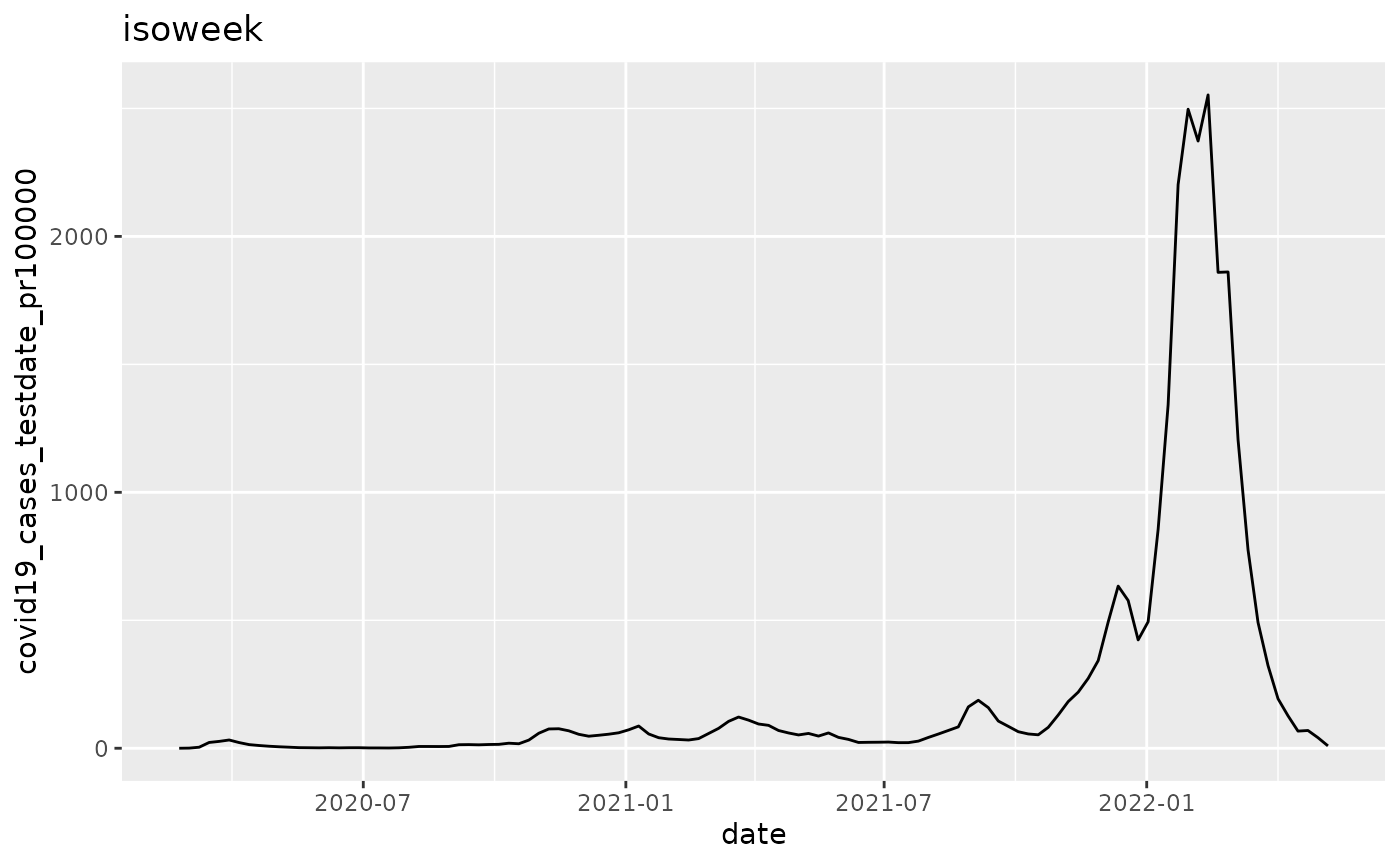
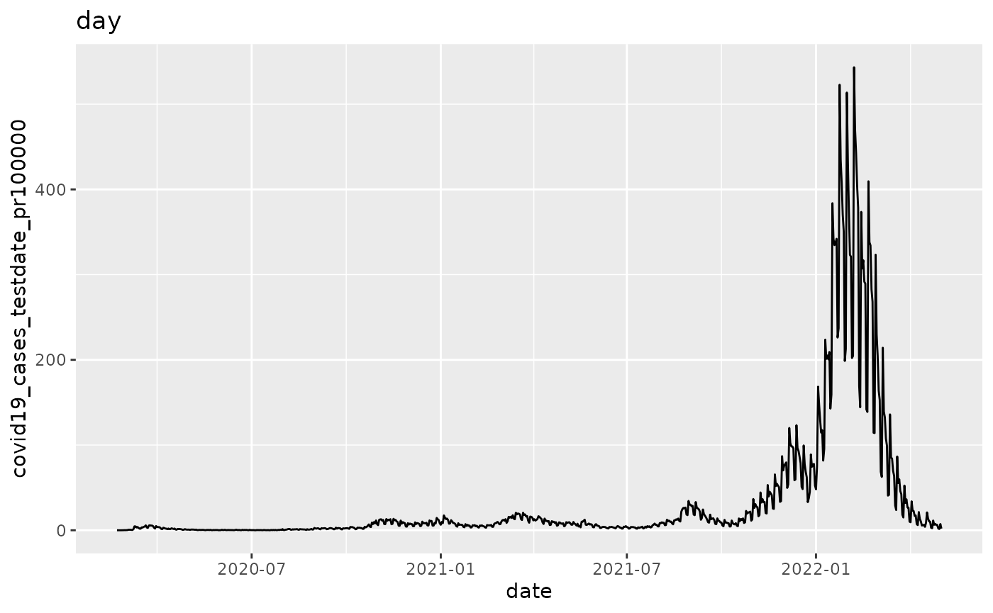
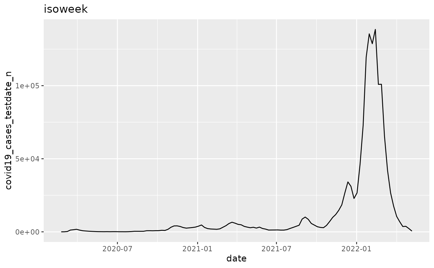
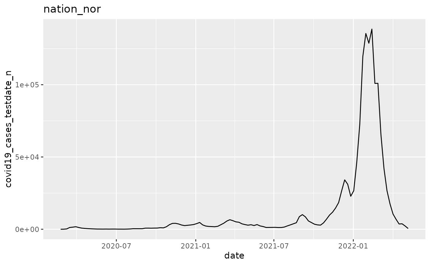
This example loops through multiple variable combinations. The combinations cross two choices:
- raw numbers of Covid-19 cases, against Covid-19 cases per 100 000 population;
- aggregation over isoweek, against aggregation over day.
The example then applies a graphing function to the data for each combination.
library(ggplot2)
library(data.table)
# We begin by defining a new plan
p <- plnr::Plan$new()
# Data function
data_fn <- function(){
return(plnr::nor_covid19_cases_by_time_location[location_code=="nation_nor"])
}
# We add sources of data
# We can add data directly
p$add_data(
name = "covid19_cases",
fn_name = "data_fn"
)
p$get_data()## $covid19_cases
## granularity_time granularity_geo country_iso3 location_code border age
## <char> <char> <char> <char> <int> <char>
## 1: day nation nor nation_nor 2020 total
## 2: day nation nor nation_nor 2020 total
## 3: day nation nor nation_nor 2020 total
## 4: day nation nor nation_nor 2020 total
## 5: day nation nor nation_nor 2020 total
## ---
## 915: isoweek nation nor nation_nor 2020 total
## 916: isoweek nation nor nation_nor 2020 total
## 917: isoweek nation nor nation_nor 2020 total
## 918: isoweek nation nor nation_nor 2020 total
## 919: isoweek nation nor nation_nor 2020 total
## sex isoyear isoweek isoyearweek season seasonweek calyear calmonth
## <char> <int> <int> <char> <char> <num> <int> <int>
## 1: total 2020 8 2020-08 2019/2020 31 2020 2
## 2: total 2020 8 2020-08 2019/2020 31 2020 2
## 3: total 2020 8 2020-08 2019/2020 31 2020 2
## 4: total 2020 9 2020-09 2019/2020 32 2020 2
## 5: total 2020 9 2020-09 2019/2020 32 2020 2
## ---
## 915: total 2022 14 2022-14 2021/2022 37 NA NA
## 916: total 2022 15 2022-15 2021/2022 38 NA NA
## 917: total 2022 16 2022-16 2021/2022 39 NA NA
## 918: total 2022 17 2022-17 2021/2022 40 NA NA
## 919: total 2022 18 2022-18 2021/2022 41 NA NA
## calyearmonth date covid19_cases_testdate_n
## <char> <Date> <int>
## 1: 2020-M02 2020-02-21 1
## 2: 2020-M02 2020-02-22 0
## 3: 2020-M02 2020-02-23 0
## 4: 2020-M02 2020-02-24 0
## 5: 2020-M02 2020-02-25 0
## ---
## 915: <NA> 2022-04-10 6888
## 916: <NA> 2022-04-17 3635
## 917: <NA> 2022-04-24 3764
## 918: <NA> 2022-05-01 2243
## 919: <NA> 2022-05-08 502
## covid19_cases_testdate_pr100000
## <num>
## 1: 0.01863037
## 2: 0.00000000
## 3: 0.00000000
## 4: 0.00000000
## 5: 0.00000000
## ---
## 915: 126.96142312
## 916: 67.00127367
## 917: 69.37903551
## 918: 41.34356447
## 919: 9.25299570
##
## $hash
## $hash$current
## [1] "0ad573d37712f0a8ab666846d1b721a1"
##
## $hash$current_elements
## $hash$current_elements$covid19_cases
## [1] "07cc51795bccaf2afebe48619ce87227"
p$add_argset_from_list(
plnr::expand_list(
variable = c("covid19_cases_testdate_n", "covid19_cases_testdate_pr100000"),
granularity_time = c("isoweek","day")
)
)
# Examine the argsets that are available
p$get_argsets_as_dt()## name_analysis index_analysis
## <char> <int>
## 1: fd701af9-9baf-4371-b715-c268a59432f7 1
## 2: 8c53e154-33b2-43f2-bc07-b7721f153668 2
## 3: e8efcb0e-69f8-4487-851c-9617c2950277 3
## 4: 803fa859-c814-4e67-9e3f-389412dec842 4
## variable granularity_time
## <list> <list>
## 1: covid19_cases_testdate_n isoweek
## 2: covid19_cases_testdate_n day
## 3: covid19_cases_testdate_pr100000 isoweek
## 4: covid19_cases_testdate_pr100000 day
# We can then add a simple analysis that returns a figure:
# To do this, we first need to create an action function
# (takes two arguments -- data and argset)
action_fn <- function(data, argset){
if(plnr::is_run_directly()){
data <- p$get_data()
argset <- p$get_argset(1)
}
pd <- data$covid19_cases[
granularity_time == argset$granularity_time
]
q <- ggplot(pd, aes_string(x="date", y=argset$variable))
q <- q + geom_line()
q <- q + labs(title = argset$granularity_time)
q
}
p$apply_action_fn_to_all_argsets(fn_name = "action_fn")
p$run_one(1)## Warning: `aes_string()` was deprecated in ggplot2 3.0.0.
## ℹ Please use tidy evaluation idioms with `aes()`.
## ℹ See also `vignette("ggplot2-in-packages")` for more information.
## This warning is displayed once per session.
## Call `lifecycle::last_lifecycle_warnings()` to see where this warning was
## generated.

p$run_one(2)
p$run_one(3)
p$run_one(4)
Multi-function plan
Use this approach when you create the output for a report, and you need multiple different tables and graphs.
library(ggplot2)
library(data.table)
# We begin by defining a new plan
p <- plnr::Plan$new()
# Data function
data_fn <- function(){
return(plnr::nor_covid19_cases_by_time_location)
}
# We add sources of data
# We can add data directly
p$add_data(
name = "covid19_cases",
fn_name = "data_fn"
)
p$get_data()## $covid19_cases
## Indices: <granularity_time__location_code>, <location_code>
## granularity_time granularity_geo country_iso3 location_code border
## <char> <char> <char> <char> <int>
## 1: day county nor county_nor03 2020
## 2: day county nor county_nor03 2020
## 3: day county nor county_nor03 2020
## 4: day county nor county_nor03 2020
## 5: day county nor county_nor03 2020
## ---
## 11024: isoweek nation nor nation_nor 2020
## 11025: isoweek nation nor nation_nor 2020
## 11026: isoweek nation nor nation_nor 2020
## 11027: isoweek nation nor nation_nor 2020
## 11028: isoweek nation nor nation_nor 2020
## age sex isoyear isoweek isoyearweek season seasonweek calyear
## <char> <char> <int> <int> <char> <char> <num> <int>
## 1: total total 2020 8 2020-08 2019/2020 31 2020
## 2: total total 2020 8 2020-08 2019/2020 31 2020
## 3: total total 2020 8 2020-08 2019/2020 31 2020
## 4: total total 2020 9 2020-09 2019/2020 32 2020
## 5: total total 2020 9 2020-09 2019/2020 32 2020
## ---
## 11024: total total 2022 14 2022-14 2021/2022 37 NA
## 11025: total total 2022 15 2022-15 2021/2022 38 NA
## 11026: total total 2022 16 2022-16 2021/2022 39 NA
## 11027: total total 2022 17 2022-17 2021/2022 40 NA
## 11028: total total 2022 18 2022-18 2021/2022 41 NA
## calmonth calyearmonth date covid19_cases_testdate_n
## <int> <char> <Date> <int>
## 1: 2 2020-M02 2020-02-21 0
## 2: 2 2020-M02 2020-02-22 0
## 3: 2 2020-M02 2020-02-23 0
## 4: 2 2020-M02 2020-02-24 0
## 5: 2 2020-M02 2020-02-25 0
## ---
## 11024: NA <NA> 2022-04-10 6888
## 11025: NA <NA> 2022-04-17 3635
## 11026: NA <NA> 2022-04-24 3764
## 11027: NA <NA> 2022-05-01 2243
## 11028: NA <NA> 2022-05-08 502
## covid19_cases_testdate_pr100000
## <num>
## 1: 0.000000
## 2: 0.000000
## 3: 0.000000
## 4: 0.000000
## 5: 0.000000
## ---
## 11024: 126.961423
## 11025: 67.001274
## 11026: 69.379036
## 11027: 41.343564
## 11028: 9.252996
##
## $hash
## $hash$current
## [1] "0306cac791d5f990073167e17ed15f9b"
##
## $hash$current_elements
## $hash$current_elements$covid19_cases
## [1] "bad75e8e213b3de3eee2b4ecbf157f46"
# Completely unique function for figure 1
p$add_analysis(
name = "figure_1",
fn_name = "figure_1"
)
figure_1 <- function(data, argset){
if(plnr::is_run_directly()){
data <- p$get_data()
argset <- p$get_argset("figure_1")
}
pd <- data$covid19_cases[
granularity_time == "isoweek"
]
q <- ggplot(pd, aes_string(x="date", y="covid19_cases_testdate_pr100000"))
q <- q + geom_line()
q <- q + facet_wrap(~location_code)
q <- q + labs(title = "Weekly covid-19 cases per 100 000 population")
q
}
# Reusing a function for figures 2 and 3
p$add_analysis(
name = "figure_2",
fn_name = "plot_epicurve_by_location",
location_code = "nation_nor"
)
# Reusing a function for figures 2 and 3
p$add_analysis(
name = "figure_3",
fn_name = "plot_epicurve_by_location",
location_code = "county_nor03"
)
plot_epicurve_by_location <- function(data, argset){
if(plnr::is_run_directly()){
data <- p$get_data()
argset <- p$get_argset("figure_2")
argset <- p$get_argset("figure_3")
}
pd <- data$covid19_cases[
granularity_time == "isoweek" &
location_code == argset$location_code
]
q <- ggplot(pd, aes_string(x="date", y="covid19_cases_testdate_n"))
q <- q + geom_line()
q <- q + labs(title = argset$location_code)
q
}
p$run_one("figure_1")
p$run_one("figure_2")
p$run_one("figure_3")